
A little bit of context
This is the tutorial material I prepared in fall 2023, for people with basic foundation of machine learning to get hands-on PyTorch quickly.
My idea behind the whole document is to teach the reader how to do full model training from the ground up and introduce each component alongside the process.
Introduction to PyTorch
![]()
- PyTorch is an open-source deep learning framework that provides a flexible and dynamic approach to building and training neural networks.
- Its popularity and widespread adoption by the research and industry communities.
- PyTorch is widely known for its ease of use, Pythonic interface, and excellent support for research-oriented tasks.
Key Technology
Dynamic computational graph
A computational graph represents the flow of data through a computational model in the form of a directed acyclic graph (DAG). It serves as a visual representation of the mathematical operations performed on input data to produce the desired output.
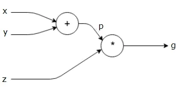
PyTorch allows for efficient and flexible model construction and dynamic control flow through its dynamic computational graph. Unlike TensorFlow, another popular deep-learning framework that employs static computational graphs, PyTorch constructs and executes the computational graph dynamically during runtime.
The dynamic nature of PyTorch’s computational graph enables greater flexibility and control flow. The graph is built on-the-fly as operations are executed, making it easier to debug and write code that involves complex or varying control flows. This feature is particularly useful for tasks that require dynamic graph construction, like recurrent neural networks or models with varying input sizes. Additionally, PyTorch’s dynamic nature facilitates seamless integration with Python control flow and external libraries. However, it’s worth noting that the dynamic construction of the graph may result in reduced performance compared to static graphs.
In contrast, TensorFlow follows a static computational graph approach where the graph is defined and compiled before execution. The graph is constructed independently of the actual data being processed, which allows for potential optimization opportunities. Once the graph is defined, it can be executed repeatedly without the need for graph construction, thereby improving performance.
TensorFlow’s static nature facilitates better graph optimization, including automatic differentiation and graph pruning. It is well-suited for scenarios where the model architecture is fixed and known in advance, with a focus on optimizing performance. However, the static nature of TensorFlow’s graph construction may limit flexibility for models with dynamic control flow or varying input sizes. Writing code with TensorFlow’s static graphs can sometimes be more complex and require additional boilerplate code.
It’s important to mention that both frameworks have evolved over time, with advancements made to enhance flexibility and efficiency. For instance, TensorFlow 2.0 introduced TensorFlow eager execution mode, which provides a dynamic execution similar to PyTorch. PyTorch also introduced TorchScript (
torch.JIT) in PyTorch 2.0 for static graph optimization.
Automatic differentiation
Overview of PyTorch Autograd Engine | PyTorch
PyTorch’s automatic differentiation is a fundamental feature that enables efficient computation of gradients for training deep learning models. It is tightly integrated with PyTorch’s dynamic computational graph, allowing for easy and efficient backpropagation of gradients through the network.
During the forward pass, PyTorch tracks operations on tensors, building a dynamic computational graph as these operations are executed. This graph records the operations and their dependencies, forming a directed acyclic graph (DAG). Each node in the graph represents an operation, and the edges represent data dependencies.
PyTorch also keeps track of the operations required for computing gradients during the forward pass. It creates a backward pass function for each operation, which calculates the gradient of the output with respect to the input tensors using the chain rule of calculus. During the backward pass, these backward pass functions are invoked to compute gradients efficiently.
The dynamic nature of PyTorch’s computational graph allows for the automatic differentiation process to be performed on a per-graph basis. Gradients are computed dynamically as the forward pass is executed. This dynamic approach offers greater flexibility and control over the model’s behavior, as the graph can change at runtime based on the data or control flow.
To perform backpropagation in PyTorch, you typically define a loss function and call the backward() method on the loss tensor. This triggers the computation of gradients using the dynamic computational graph and the chain rule, updating the gradients of all the model’s parameters. These gradients can then be used to update the model’s weights using an optimizer, such as stochastic gradient descent (SGD).
Overall, PyTorch’s automatic differentiation capability, combined with its dynamic computational graph, simplifies the process of computing gradients and enables efficient backpropagation for training deep learning models.
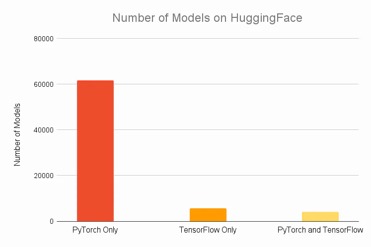
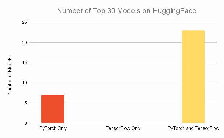
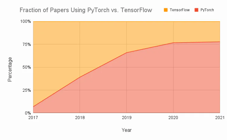
Comparison with Other
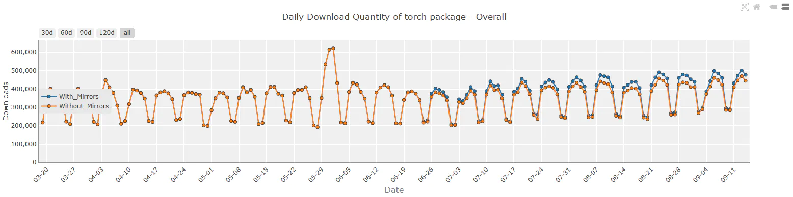
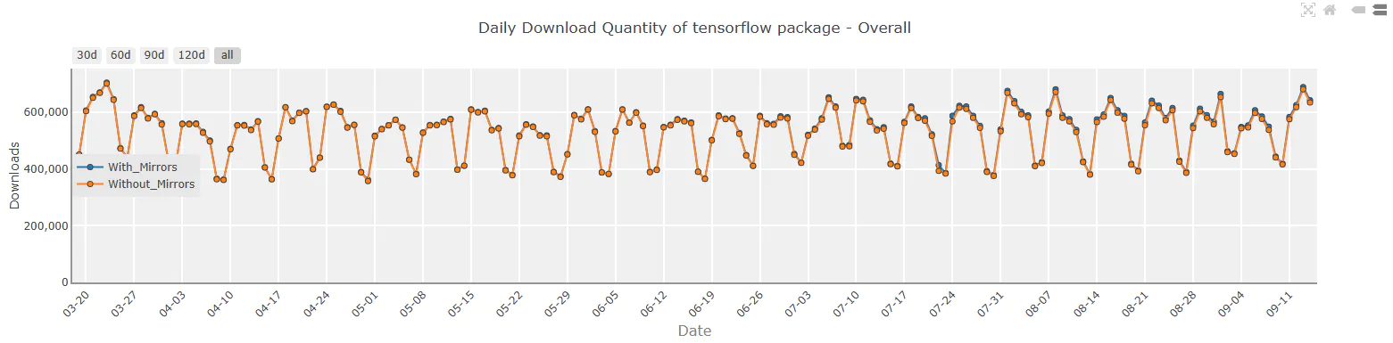
These figures show the usage of DL frameworks based on PyPI downloads, the number of models available on HuggingFace, and the changes in publications over time.
How to use PyTorch
To use PyTorch, you have different options depending on the environment you are working in.
Online Computation Resource
If you are using platforms like Kaggle, Google Colab, or any other similar environment, you typically don’t need to set up the PyTorch environment explicitly. These platforms provide a containerized environment with the necessary computational resources and basic environment already installed.
Your Own Machine
If you want to work on your own machine, you can follow these steps:
- Ensure you have Python installed on your machine. You can use Anaconda or Miniconda Python distributions: Anaconda/Miniconda Miniconda — miniconda documentation
- To install PyTorch, you can either use pip or conda: Start Locally | PyTorch
pip install torch torchvision torchaudio --index-url https://download.pytorch.org/whl/cpu
# or
conda install pytorch torchvision torchaudio cpuonly -c pytorch
This command will download and install the CPU version of PyTorch.
With GPU
If you have a GPU and want to utilize its power for accelerated computations, make sure you have a GPU that supports CUDA 11 or later.
- CUDA Environment: CUDA Zone - Library of Resources | NVIDIA Developer
- To install the GPU version of PyTorch, use pip with the following command:
pip3 install torch torchvision torchaudio --index-url https://download.pytorch.org/whl/cu117
These steps will help you set up PyTorch based on your specific requirements and environment.
Tensors and Operations
Tensor
Tensors are a specialized data structure that are very similar to arrays and matrices (multi-dimensional array). In PyTorch, we use tensors to encode the inputs and outputs of a model, as well as the model’s parameters.
Tensor can have different data types such as float, integer, or boolean, which is similar to NumPy’s ndarray and, except that tensors can run on GPUs or other hardware accelerators. In fact, tensors and NumPy arrays can often share the same underlying memory, eliminating the need to copy data. Tensors are also optimized for automatic differentiation.
Initializing a Tensor
- Direct: You can initialize a tensor of a specific size with all elements set to zero using the torch.zeros() function.
# Initialize a tensor of size 2x3 with all elements set to zero
tensor_a = torch.zeros(2, 3)
print(tensor_a)
- From NumPy: You can create a NumPy array and then initialize a tensor from it using the
torch.from_numpy()function.
import numpy as np

# Create a NumPy array
numpy_array = np.array([[1, 2, 3], [4, 5, 6]])

# Initialize a tensor from the NumPy array
tensor_b = torch.from_numpy(numpy_array)
print(tensor_b)
- From another tensor: You can create a new tensor from an existing tensor using the
torch.tensor()function.
# From another tensor
tensor_c = torch.tensor([[1, 2, 3], [4, 5, 6]])

# When you use torch.tensor(), you create a new tensor
# without any connection to the original tensor's computational
# graph or gradient history. This means that the new tensor will
# not have any gradients associated with it, and it will not
# participate in any future gradient calculations or
# backpropagation.

# tensor_d = torch.tensor(tensor_c)
# print(tensor_d)

tensor_e = tensor_c.clone().detach()

print(tensor_e)
- Fill in random or constant values: You can initialize a tensor with random values. You can also initialize a tensor with constant values using
torch.full().
# Fill in random or constant values
tensor_f = torch.rand(3, 2)  # Uniform Distribution
print(tensor_f)

tensor_g = torch.randn(2, 2)  # Normal Distribution
print(tensor_g)

tensor_h = torch.full((3, 3), 7)  # Filled with constant value
print(tensor_h)
Attributes of a Tensor
Tensors in PyTorch have attributes that provide information about their shape, data type, device, and gradient requirements. Some commonly used attributes include:
- Shape: It represents the size of each dimension of the tensor. You can access it using the shape attribute or the
size()method. For example,tensor.shapeortensor.size()will return the shape of the tensor. - Datatype: It indicates the data type of the elements stored in the tensor. PyTorch supports various data types such as
torch.float32,torch.int64,torch.bool, etc. You can access the data type of a tensor using thedtypeattribute. - Device: It specifies the device (CPU or GPU) on which the tensor is stored. You can use the device attribute to check if the tensor is on the CPU or GPU.
requires_grad: This attribute indicates whether the tensor requires gradient computation for automatic differentiation. By default, tensors created directly from data do not require gradients. You can enable gradient tracking by settingrequires_grad=Trueon a tensor.
tensor = torch.zeros(2, 3, 4)
print(f"tensor shape: {tensor.shape}")  # This is a attribute, not function
print(f"tensor size: {tensor.size()}")

print(f"tensor dtype: {tensor.dtype}")
tensor = torch.zeros(2, 3, dtype=torch.float64)  # explicite define the dtype for tensor
print(f"tensor dtype: {tensor.dtype}")

# tensor = torch.zeros(2, 3).to('cuda')
print(f"tensor device: {tensor.device}")
Operations
Tensors in PyTorch support a wide range of operations for manipulating and performing computations on the data they contain. These operations include arithmetic operations, linear algebra, matrix manipulation (such as indexing and slicing), and more. You can refer to the PyTorch documentation for a comprehensive list of tensor operations.
Some examples of tensor operations include:
- Indexing and slicing: Tensors can be indexed and sliced using similar syntax as NumPy arrays.
- Joining tensors: Tensors can be concatenated or stacked along different dimensions.
- Reshaping: Tensors can be reshaped to have a different shape but the same data.
- Arithmetic operations: Tensors support element-wise addition, multiplication, and matrix multiplication.
tensor = torch.tensor([[1, 2, 3], [4, 5, 6]])

# Indexing
print(tensor[0, 1])  # Output: 2

# Slicing
print(tensor[:, 1:])  # Output: tensor([[2, 3], [5, 6]])

# Joining tensors
tensor1 = torch.tensor([[1, 2], [3, 4]])
tensor2 = torch.tensor([[5, 6], [7, 8]])

# Concatenation
concatenated = torch.cat((tensor1, tensor2), dim=0)  # Concatenate along dimension 0
print(concatenated)

# Stacking
stacked = torch.stack((tensor1, tensor2), dim=0)  # Stack along new dimension 0
print(stacked)

# Reshape: Returns a tensor with the same data but a different shape.
tensor = torch.tensor([[1, 2], [3, 4]])
reshaped = torch.reshape(tensor, (4,))
print(reshaped)
Arithmetic operations
tensor1 = torch.tensor([[1, 2], [3, 4]])
tensor2 = torch.tensor([[5, 6], [7, 8]])

# Element-wise addition
result = tensor1 + tensor2
print(result)

# Element-wise multiplication
result = tensor1 * tensor2
print(result)

# Matrix Multiplication
result = torch.matmul(tensor1, tensor2)
print(result)
Building Neural Networks
nn.Module Class
The nn.Module class serves as a base class for all neural network modules in PyTorch. It is used to define the architecture and behavior of the network. This class provides a convenient way to organize the parameters of a model and define the forward pass computation. To create your own neural network using nn.Module, you need to define a subclass of nn.Module and override two key methods: __init__ and forward. The __init__ method is used to define the layers and modules of your network, while the forward method specifies the forward pass computation.
import torch
import torch.nn as nn

class MyNetwork(nn.Module):
    def __init__(self):
        super(MyNetwork, self).__init__()
        # Define the layers and modules of your network
        self.fc1 = nn.Linear(10, 5)
        self.fc2 = nn.Linear(5, 2)

    def forward(self, x):
        # Define the forward pass computation
        x = self.fc1(x)
        x = self.fc2(x)
        return x
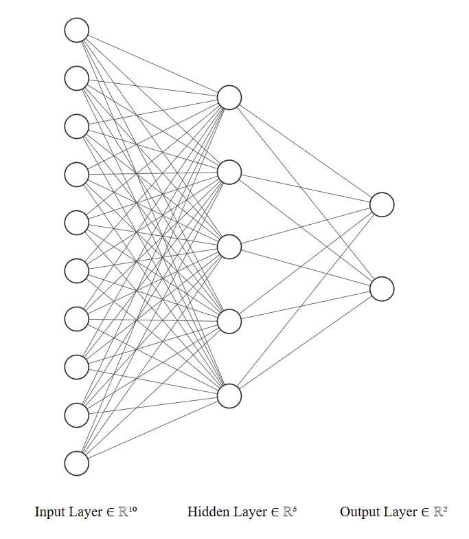
In the __init__ method, you can define any layers or modules you need for your network. In this example, we define two fully connected layers (nn.Linear) with specified input and output sizes.
In the forward method, you specify the sequence of operations that will be applied to the input x during the forward pass. In this example, we apply the first linear layer (self.fc1), followed by the second linear layer (self.fc2).
batch_size = 1
in_features = 10

model = MyNetwork()

input_data = torch.randn(batch_size, in_features)
output = model(input_data)

print(f"input: {input_data}\noutput: {output}")
In this example, we first instantize the network we just defined. And setup the input_data which is a tensor representing the input to your network. You can pass this input tensor to your network instance (model) to obtain the output tensor (output). The forward method of your network will be automatically called, executing the forward pass computation defined earlier.
Predefined Layers
PyTorch’s nn module provides a wide range of predefined layers that you can use to build your neural networks. Just like the nn.Linear and nn.ReLU we just use. Here are some commonly used layers:
nn.Linear: This layer implements a fully connected (linear) operation. It applies a linear transformation to the input data, where each input element is multiplied by a weight and summed with a bias term.nn.Conv2d: This layer performs 2D convolutional operations on input data, commonly used in image processing tasks. It applies a set of learnable filters (kernels) to the input tensor to extract local features. nn.Dropout: This layer implements dropout regularization, which randomly sets input elements to zero during training. Dropout helps prevent overfitting by reducing the interdependencies between neurons.nn.BatchNorm2d: This layer performs batch normalization along the channels of a 2D input tensor. It normalizes the input by subtracting the mean and dividing by the standard deviation, which helps stabilize and accelerate the training process.nn.ReLU: This activation function applies the Rectified Linear Unit (ReLU) element-wise to the input tensor. ReLU sets negative values to zero and keeps positive values unchanged.nn.Softmax: This activation function applies the softmax operation to the input tensor, which normalizes the tensor into a probability distribution over the classes. It is commonly used for multi-class classification problems.
class MyNetwork(nn.Module):
    def __init__(self, in_channels, out_classes):
        super(MyNetwork, self).__init__()
        self.conv = nn.Conv2d(in_channels, 64, kernel_size=3, padding=1)
        self.batchnorm = nn.BatchNorm2d(64)
        self.relu = nn.ReLU()
        self.dropout = nn.Dropout(p=0.2)

        self.fc1 = nn.Linear(64 * 28 * 28, 128)
        self.fc2 = nn.Linear(128, out_classes)

        self.softmax = nn.Softmax(dim=1)

    def forward(self, x):
        x = self.conv(x)
        x = self.batchnorm(x)
        x = self.relu(x)
        x = self.dropout(x)

        x = x.view(x.size(0), -1)  # Flatten the tensor

        x = self.fc1(x)
        x = self.relu(x)
        x = self.dropout(x)

        x = self.fc2(x)
        x = self.softmax(x)

        return x
Model Summary and Parameters
model = MyNetwork(in_channels=1, out_classes=10)

# Print the network structure
print(model)

# Calculate the parameter count
total_params = sum(p.numel() for p in model.parameters() if p.requires_grad)
print(f"Total parameters: {total_params}")

"""
Output:

MyNetwork(
  (conv): Conv2d(3, 64, kernel_size=(3, 3), stride=(1, 1), padding=(1, 1))
  (batchnorm): BatchNorm2d(64, eps=1e-05, momentum=0.1, affine=True, track_running_stats=True)
  (relu): ReLU()
  (dropout): Dropout(p=0.2, inplace=False)
  (fc1): Linear(in_features=50176, out_features=128, bias=True)
  (fc2): Linear(in_features=128, out_features=10, bias=True)
  (softmax): Softmax(dim=1)
)
Total parameters: 6425866
"""
There is a convenient package called torchsummary that you can use to calculate the total number of parameters in a PyTorch model. Here’s how you can use it:
from torchsummary import summary

# Instantiate the network
model = MyNetwork(in_channels=1, out_classes=10)
model = model.to("cuda:0")
# Print the model summary
summary(model, (1, 28, 28))  # Provide an example input size

"""
Output:

----------------------------------------------------------------
        Layer (type)               Output Shape         Param #
================================================================
            Conv2d-1           [-1, 64, 28, 28]           1,792
       BatchNorm2d-2           [-1, 64, 28, 28]             128
              ReLU-3           [-1, 64, 28, 28]               0
           Dropout-4           [-1, 64, 28, 28]               0
            Linear-5                  [-1, 128]       6,422,656
              ReLU-6                  [-1, 128]               0
           Dropout-7                  [-1, 128]               0
            Linear-8                   [-1, 10]           1,290
           Softmax-9                   [-1, 10]               0
================================================================
Total params: 6,425,866
Trainable params: 6,425,866
Non-trainable params: 0
----------------------------------------------------------------
Input size (MB): 0.01
Forward/backward pass size (MB): 1.53
Params size (MB): 24.51
Estimated Total Size (MB): 26.06
----------------------------------------------------------------
"""
Dataset and DataLoader
PyTorch Dataset represents a dataset of input samples and their corresponding labels, while PyTorch DataLoader is responsible for efficiently loading the data from the dataset during training or inference.
Dataset Class
The PyTorch torch.utils.data.Dataset class is a base class that you can inherit from to create your custom dataset.
To create a dataset in PyTorch, you need to override the following methods of the Dataset class:
__len__: Returns the total number of data samples in the dataset.__getitem__: Retrieves a specific data sample from the dataset, given its index.
import torch
from torch.utils.data import Dataset

class CustomDataset(Dataset):
    def __init__(self, data):
        self.data = data

    def __len__(self):
        return len(self.data)

    def __getitem__(self, index):
        sample = self.data[index]
        # Implement any necessary preprocessing or data transformations here
        # Return the preprocessed sample
        return sample

# Create an instance of your custom dataset
data = [1, 2, 3, 4, 5]
dataset = CustomDataset(data)

# Access individual data samples
sample = dataset[0]
print(sample)  # Output: 1
Built-in Datasets
PyTorch provides several built-in datasets through the torchvision.datasets module. These datasets are commonly used for computer vision tasks. Here are some of the popular built-in datasets available in PyTorch:
- MNIST: Handwritten digit dataset.
- CIFAR10 and CIFAR100: Small images dataset with 10 and 100 classes, respectively.
- ImageNet: Large-scale image dataset with 1000 classes.
- FashionMNIST: Fashion product images dataset.
- COCO: Common Objects in Context dataset for object detection, segmentation, and captioning.
- VOC: Visual Object Classes dataset for object detection, segmentation, and classification.
- LSUN: Large-scale Scene Understanding dataset for scene classification and generation.
- SVHN: Street View House Numbers dataset.
- STL10: Small images dataset with 10 classes.
- CelebA: Large-scale celebrity faces dataset.
To use these built-in datasets in PyTorch, you need to follow these steps:
from torchvision import datasets

dataset = datasets.MNIST(root='./data', train=True, download=True)

# Access the samples
sample = dataset[1]

import matplotlib.pyplot as plt  # Visualize
plt.figure(figsize=(3,3))
plt.imshow(sample[0])
plt.show()
Transformations
Transformations in PyTorch are operations applied to data samples in a dataset. They are commonly used to preprocess or augment the data before feeding it into a machine learning model. PyTorch provides the torchvision.transforms module, which offers a variety of predefined transformations for computer vision tasks. Here are some commonly used transformations:
-
ToTensor(): Converts a PIL image or numpy array to a PyTorch tensor. It also scales the pixel values between 0 and 1. -
Normalize(mean, std): Normalizes a tensor by subtracting the mean and dividing by the standard deviation. The mean and std arguments specify the channel-wise means and standard deviations. -
Resize(size): Resizes the input PIL image to the specified size. It can take a single integer as an argument to resize the image’s shorter side while maintaining its aspect ratio. -
CenterCrop(size): Crops the center portion of the image to the specified size. -
RandomCrop(size): Randomly crops the input image to the specified size. -
RandomHorizontalFlip(): Randomly flips the input image horizontally with a probability of 0.5. -
RandomRotation(degrees): Rotates the input image by a random angle within the specified range. -
RandomResizedCrop(size): Randomly crops and resizes the input image to the specified size.
from torchvision import transforms

# Define the transformations
transform = transforms.Compose([
    transforms.CenterCrop(20),  # Crops the given image at the center.
    transforms.Resize(28),  # Resize the input image to 28*28
    # transforms.RandomHorizontalFlip(),  # Randomly flip horizontally
    transforms.ToTensor(),  # Convert PIL image to tensor
    transforms.Normalize((0.5,), (0.5,))  # Normalize tensor
])

# Create an instance of the dataset with transformations
dataset = datasets.MNIST(root='./data', train=True, download=True, transform=transform)
What is DataLoader and how to use
In PyTorch, a DataLoader is an iterable that provides an interface to efficiently load data from a dataset during training or evaluation. It handles batch loading, shuffling, and other useful functionalities to facilitate the training process. The DataLoader takes a dataset as input and returns batches of data samples and their corresponding labels.
The relationship between a dataset and a DataLoader is that the DataLoader wraps the dataset and provides an interface to access the data in batches. It abstracts away the details of data loading and allows you to focus on training your model.
To use a DataLoader with the dataset you defined, you can follow these steps:
import torch
from torch.utils.data import DataLoader

dataset = CustomDataset(data)

dataloader = DataLoader(dataset, batch_size=32, shuffle=True)

for batch_data, batch_labels in dataloader:
    # Use the batch_data and batch_labels for training or evaluation
    # ...

    # Clear gradients, perform backward pass, update model parameters, etc.
    # ...
Training and Optimization
Splitting data into training, validation, and test sets The common method we use for the dataset split is from sklearn
from sklearn.model_selection import train_test_split  dataset = CustomDataset(data)

# Split the data into train, validation, and test sets
train_data, test_data = train_test_split(dataset, test_size=0.2, random_state=42)
train_data, val_data = train_test_split(train_data, test_size=0.2, random_state=42)
In the example above, the dataset is split into 80% training data and 20% test data. Then, the training data is further split into 80% for training and 20% for validation.
Once you have split your data into training, validation, and test sets, you can construct separate data loaders for each set.
# Define batch size
batch_size = 32

# Create data loaders for training, validation, and test sets
train_loader = DataLoader(train_data, batch_size=batch_size, shuffle=True)
val_loader = DataLoader(val_data, batch_size=batch_size)
test_loader = DataLoader(test_data, batch_size=batch_size)
In the code above, train_data, val_data, and test_data represent the respective splits of your dataset. The batch_size parameter specifies the number of samples in each batch. You can adjust this value based on your computational resources and model requirements.
The DataLoader class from PyTorch is used to create the data loaders. The shuffle=True argument is passed to the training loader to randomly shuffle the samples in each epoch, which helps in improving the model’s generalization.
Defining loss functions (e.g., cross-entropy, mean squared error)
After defining the data loader and model in a deep learning task, the next steps typically involve defining the loss function and optimizer. Here’s a general outline of how to do that:
The loss function measures the discrepancy between the predicted output of your model and the true labels. The choice of loss function depends on the specific task you are working on. Some common loss functions include:
- Mean Squared Error (MSE): Suitable for regression tasks where the output is continuous.
- Binary Cross-Entropy: Used for binary classification tasks where the output is a probability between 0 and 1.
- Categorical Cross-Entropy: Appropriate for multi-class classification problems where the output is a probability distribution over multiple classes.
# loss_fn = nn.MSELoss()
# loss_fn = nn.BCELoss()
loss_fn = nn.CrossEntropyLoss()
# loss_fn = nn.KLDivLoss()
Choosing and configuring optimizers (e.g., SGD, Adam)
The optimizer is responsible for updating the model’s parameters based on the computed gradients during the backpropagation process. It adjusts the parameters in the direction that minimizes the loss function. One commonly used optimizer is Stochastic Gradient Descent (SGD), but there are many other variants available, such as Adam, RMSprop, and Adagrad. PyTorch provides various optimizers in the torch.optim module. To use an optimizer, you typically need to pass the model parameters and specify the learning rate. Here’s an example of defining an optimizer:
import torch.optim as optim

# optimizer = optim.SGD(model.parameters(), lr=0.001)
# Or
optimizer = optim.Adam(model.parameters(), lr=0.001)
Do Training
Once you have defined the model, data loader, loss function, and optimizer, you can proceed with training your model and calculating metrics for each batch and epoch. Here’s an overview of the steps involved:
Training Loop: Iterate over your data for a specified number of epochs. In each epoch, iterate over the batches of data provided by the data loader. Here’s an example of a training loop:
device = 'cuda' if torch.cuda.is_available() else 'cpu'
model = model.to(device)
loss_fn = loss_fn.to(device)

import torch.nn.functional as F

def metric(batch_predictions, batch_labels):
    # Convert the predictions and labels to numpy arrays
    _, predicted_labels = torch.max(batch_predictions, dim=1)
    correct_predictions = (predicted_labels == batch_labels).sum().item()
    # Calculate the prediction error
    accuracy = correct_predictions / len(batch_labels)
    return accuracy

num_epochs = 10
for epoch in range(num_epochs):
    epoch_loss = 0.0
    epoch_metric = 0.0
    batch_count = 0

    # Iterate over the batches in the dataloader
    for batch in train_loader:
        # Clear gradients from previous iteration
        batch_data, batch_labels = batch[0], batch[1]
        batch_data = batch_data.to(device)
        batch_labels = batch_labels.to(device)
        # print(batch_data.size())
        optimizer.zero_grad()

        # Forward pass
        batch_predictions = model(batch_data)
        # print(batch_predictions)

        # Calculate loss
        loss = loss_fn(batch_predictions, batch_labels)
        epoch_loss += loss.item()

        # Backward pass
        loss.backward()
        optimizer.step()

        # Calculate and record metrics
        batch_metric = metric(batch_predictions, batch_labels)
        epoch_metric += batch_metric

        batch_count += 1

    # Calculate average loss and metric for the epoch
    avg_epoch_loss = epoch_loss / batch_count
    avg_epoch_metric = epoch_metric / batch_count

    # Print or log the metrics for analysis
    print(f"Epoch {epoch+1} - Loss: {avg_epoch_loss:.4f} - Metric: {avg_epoch_metric:.4f}")
You’ll typically follow these steps:
- Iterate over the training dataset for a specific number of epochs.
- Within each epoch, iterate over the batches of the dataset.
- Perform the forward pass through the model to obtain predictions.
- Calculate the loss using the defined loss function.
- Perform the backward pass and update the model parameters using the optimizer.
- Calculate and record the desired metrics for analysis.
- Within each epoch, iterate over the batches of the dataset.
Saving and Loading Models
To save a trained model in PyTorch, you can use the torch.save() function. This function allows you to save various components of the model, including the model’s architecture, parameters, optimizer state, and any additional information you want to store.
torch.save(model, 'saved_model.pth')
In this example, the model object is saved in a file called “saved_model.pth”. This file will contain the entire model, including its architecture, parameters, and other associated information.
When you load the saved model, you can use the torch.load() function. Here’s an example of how to load the saved model:
loaded_model = torch.load('saved_model.pth')
loaded_model = loaded_model.to(device)
# Print the model summary
summary(loaded_model, (1, 28, 28))  # Provide an example input size
The torch.load() function returns the model object, which you can assign to a variable (loaded_model in this case). After loading, you can use the loaded model for inference, evaluation, or further training.
Note that when you save the entire model using torch.save(), it saves the complete state of the model, including all parameters and buffers. However, it does not save the optimizer state by default. If you want to save and load the optimizer state as well, you can save it separately or include it in a dictionary along with the model.
# Save model and optimizer together
checkpoint = {
    'model_state_dict': model.state_dict(),
    'optimizer_state_dict': optimizer.state_dict()
}
torch.save(checkpoint, 'saved_model-w-optimizer.pth')
To load the model and optimizer together, you can use torch.load() and then access the saved states:
checkpoint = torch.load('saved_model-w-optimizer.pth')
opt_model = MyNetwork(in_channels=1, out_classes=10)
opt_optimizer = optim.Adam(opt_model.parameters(), lr=0.001)
opt_model.load_state_dict(checkpoint['model_state_dict'])
opt_optimizer.load_state_dict(checkpoint['optimizer_state_dict'])
Transfer Learning
In PyTorch, you can use predefined models from the torchvision.models module, which provides a collection of popular pre-trained models for tasks such as image classification, object detection, and segmentation (Huggingface for NLP, LLM, and Multi-modal). These models are trained on large datasets like ImageNet and have learned useful features that can be leveraged for various computer vision tasks.
Load Models and Pre-trained weights
To use a predefined model and download its pre-trained parameters, you can follow these steps:
Import the necessary modules, and load a model:
import torchvision.models as models

model = models.resnet50(weights=models.ResNet50_Weights.IMAGENET1K_V1)
In this example, the ResNet-50 model is loaded with pre-trained weights. You can choose different models such as ResNet-18, VGG-16, etc. Here is the full model list: Models and pre-trained weights — Torchvision 0.15 documentation (pytorch.org)
Modify model for your task
After loaded such model with pre-trained parameters, you can use them just like the model you defined, but you have to know that the model is design for a specific tasks, which may not align with yours. So if you want to use the model on your task and fully utilize the pretrain effort, you can change the model and do transfer learning (fine-tuning). What you need to do is replacing or fine-tuning the last fully connected layer. For ResNet model the last layer typically corresponds to the classification layer for ImageNet’s 1000 classes. If your task has a different number of classes, you need to adapt the last layer accordingly. For example:
num_classes = 10
model.fc = torch.nn.Linear(model.fc.in_features, num_classes)
In this example, the last fully connected layer (model.fc) is replaced with a new linear layer that has num_classes output units.
Depending on your task and the amount of available data, you may choose to freeze some layers to prevent their weights from being updated during training. This is particularly useful when you have limited data or when the pre-trained model is already well-suited to your task. For example, to freeze all layers except the last one:
for param in model.parameters():
    param.requires_grad = False
model.fc.weight.requires_grad = True
model.fc.bias.requires_grad = True
In this example, all parameters (requires_grad) are set to False except for the weights and biases of the last fully connected layer (model.fc).
With these steps, you can use a pre-trained model, download its pre-trained parameters, and modify it to suit your specific task. Once you’ve made the necessary modifications, you can train the model on your own dataset or use it for inference.
PS: The layer naming is not fully aligned for all model, like the Transformer model have a different name and structure for the output layer, you need to look in to the model first before the modification.
GPU Acceleration
GPU acceleration in PyTorch refers to leveraging the computational power of Graphics Processing Units (GPUs) to speed up training and inference processes. GPUs are highly parallel processors capable of performing multiple calculations simultaneously, making them well-suited for tasks involving large-scale matrix computations, such as deep learning.
To utilize CUDA and GPU-enabled devices in PyTorch, you need to ensure that you have the appropriate hardware (an NVIDIA GPU) and the necessary software dependencies installed, including CUDA Toolkit and cuDNN. Once you have these prerequisites set up, you can follow these steps to move tensors and models to the GPU for faster computation:
device = torch.device("cuda" if torch.cuda.is_available() else "cpu")
This code snippet checks if CUDA is available and assigns the device accordingly. If CUDA is available, the device will be set to "cuda"; otherwise, it will fall back to the CPU.
- Move tensors to the GPU:
tensor = tensor.to(device)
This line of code moves a PyTorch tensor to the GPU by calling the to() method and passing the device as an argument. After this operation, computations involving this tensor will be performed on the GPU.
- Move models to the GPU:
model = model.to(device)
Similarly, you can move an entire PyTorch model to the GPU using the to() method. This ensures that all model parameters and computations are performed on the GPU.
- Ensure inputs are also on the GPU:
If you’re passing inputs to the model during training or inference, make sure to move those tensors to the GPU as well. For example:
input_data = input_data.to(device)
By moving tensors and models to the GPU, PyTorch automatically utilizes the GPU’s computational power, leading to faster computations compared to running on the CPU. It’s important to note that not all operations are automatically GPU-accelerated. PyTorch provides GPU-accelerated implementations for most common operations, but some custom operations may require manual implementation for GPU compatibility.
When using a GPU, it’s also essential to manage GPU memory appropriately, especially when working with large models or batches of data. You may need to optimize your code to minimize memory usage, such as using gradient accumulation or batch splitting techniques.
Remember to perform necessary operations on the same device (CPU or GPU) to avoid unnecessary data transfers between devices, as it can negatively impact performance.
Addition Topics
Random Seed
The random seed is a crucial parameter when working with random number generation in PyTorch or any other deep learning framework. It is used to initialize the pseudorandom number generator (PRNG) algorithm, which is responsible for generating random numbers during model training.
By setting a specific random seed, you can ensure reproducibility of your experiments. When the same random seed is used, the sequence of random numbers generated by the PRNG will be the same across multiple runs. This is important because deep learning models often involve random initialization of weights, dropout, data shuffling, and other stochastic operations. Reproducibility allows you to compare different model configurations, debug code, and share results with others.
To preserve determinism when working with random seeds in PyTorch, there are a few key points to keep in mind:
- Setting the seed: Before initializing your model or performing any random operations, set the random seed using the
torch.manual_seed(seed)function, whereseedis an integer value. You can also set the random seed for numpy and other libraries if they are used in conjunction with PyTorch. - GPU considerations: If you are using GPUs for training, be aware that additional steps may be necessary to ensure deterministic results. For example, you can use
torch.backends.cudnn.deterministic = Trueandtorch.backends.cudnn.benchmark = Falseto disable certain GPU optimizations that introduce non-determinism. - NumPy interactions: If your code involves interactions between PyTorch and NumPy, be mindful that both libraries have their own random number generators. To maintain determinism, set the random seed for both libraries using
np.random.seed(seed)andtorch.manual_seed(seed). - Non-deterministic operations: While setting a random seed helps control the sources of randomness, some operations in PyTorch may still be non-deterministic, even with a fixed seed. Examples include certain GPU operations or multi-threaded code. In such cases, achieving full determinism may not be possible.
- Library versions: Ensure that you are using the same version of PyTorch and related libraries across different runs. Changes in library versions or underlying algorithms could affect the reproducibility of results, even with the same random seed.
- By being mindful of these considerations and setting the random seed appropriately, you can increase the reproducibility of your PyTorch model training experiments. Your can check more about reproducibility from Torch Document: Reproducibility — PyTorch 2.0 documentation
DataLoader Worker
When using a data loader in frameworks like PyTorch or TensorFlow, you often have the option to specify the number of worker processes to use for data loading. These worker processes, also known as data loading threads, are responsible for asynchronously loading and preprocessing data in parallel to speed up the overall data loading process.
The correct number of worker processes to use depends on various factors, including the characteristics of your dataset, the available computational resources, and the specific requirements of your training or inference pipeline. In general, increasing the number of worker processes can help speed up data loading, especially when the data loading and preprocessing operations are computationally expensive. However, there are practical limitations to consider, such as the number of CPU cores available and the memory requirements of each worker.